MS2 Extraction

With MS1 features of interest determined by peak detection, corresponding tandem mass spectra, if available, must be extracted and assigned to the MS1 parent ion feature. For data independent acquisition, we use non-m/z dimensions to assign fragments; for instance, drift time and retention time are used to match fragments in LC-IMS-MS/MS. These additional separations enable better attribution of MS2 ions to parent ions, a form of deconvolution inherent in the acquisition, but convolution artifacts can still occur.

Explicit, algorithmic deconvolution has been implemented such that MS1 and MS2 features overlapping in non-m/z separation dimensions are disambiguated to minimize false assignments. In this form of deconvolution, the profile(s) of non-m/z separation dimensions are used to identify only those ions in the MS2 with distributions that correspond to the precursor ion distribution. This technique simultaneously excludes MS2 ions arising from noise or chemical background, while also attributing MS2 ions only to precursor ions with similar separation distributions.

Drift Time Offset

In these data, the mass analyzer connected to the drift tube acts in itself like a miniature ion mobility separation aparatus, wherein separations are a function of both the m/z of the ion as well as the voltage applied in the collision cell. As such, when an ion in the MS1 experiences a collsion energy of 0 eV, while its fragment ions experience higher collision energies (in this example, 20 eV), their reported drift times will be “offset” proportional to the collision energy difference and neutral loss. That is, the MS2 ions, under higher voltage, will travel faster than the corresponding MS1 ions, and thus will have a lower reported drift time.

To demonstrate, we’ll visualize the drift time dimension of a selected precursor and its putative MS2 fragments.

import deimos
import matplotlib.pyplot as plt
import numpy as np

ms1 = deimos.load('example_data.h5', key='ms1', columns=['mz', 'drift_time', 'retention_time', 'intensity'])
ms2 = deimos.load('example_data.h5', key='ms2', columns=['mz', 'drift_time', 'retention_time', 'intensity'])

ms1 = deimos.threshold(ms1, threshold=100)
ms2 = deimos.threshold(ms2, threshold=100)

# get maximal data point
mz_i, dt_i, rt_i, intensity_i = ms1.loc[ms1['intensity'] == ms1['intensity'].max(), :].values[0]

# subset the raw data
precursor = deimos.slice(ms1,
                       by=['mz', 'drift_time', 'retention_time'],
                       low=[mz_i - 0.1, dt_i - 1, rt_i - 1],
                       high=[mz_i + 0.2, dt_i + 1, rt_i + 2])

# putative fragments
fragment_profile = deimos.slice(ms2,
                                by=['drift_time', 'retention_time'],
                                low=[dt_i - 1.5, rt_i - 1],
                                high=[dt_i + 1, rt_i + 2])

fragment_dt = deimos.collapse(fragment_profile, keep='drift_time').sort_values(by='drift_time')
precursor_dt = deimos.collapse(precursor, keep='drift_time').sort_values(by='drift_time')

fig, ax = plt.subplots(1, dpi=150, facecolor='w')

ax.fill_between(precursor_dt['drift_time'],
                precursor_dt['intensity'] / precursor_dt['intensity'].max(),
                color='C0', alpha=0.4, label='Precursor')

ax.fill_between(fragment_dt['drift_time'],
                fragment_dt['intensity'] / fragment_dt['intensity'].max(),
                color='C3', alpha=0.4, label='Fragments')

ax.set_xlabel('Drift Time', fontweight='bold')
ax.set_ylabel('Normalized Intensity', fontweight='bold')
ax.set_ylim(0, None)
ax.legend()

plt.tight_layout()
plt.show()

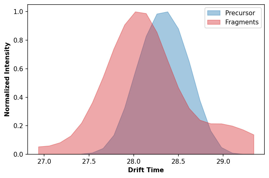
Fortunately, fragment offset correction is handled within the DEIMoS’s deconvolution module. The model to correct for offset was built from TuneMix data acquired on both our IMS instrument and an Orbitrap. Orbitrap MS1:MS2 pairs were used as ground truth, matching drift time information from the same MS1:MS2 pairs collected with IMS. Ordinary least squares (OLS) regression was used to relate model inputs to predicted values. The following model is supplied as default, but may be swapped out as needed.

def offset_correction_model(dt_ms2, mz_ms2, mz_ms1, ce=0,
                            params=[1.02067031, -0.02062323,  0.00176694]):
    # Cast params as array
    params = np.array(params).reshape(-1, 1)

    # Convert collision energy to array
    ce = np.ones_like(dt_ms2) * np.log(ce)

    # Create constant vector
    const = np.ones_like(dt_ms2)

    # Sqrt
    mu_ms1 = np.sqrt(mz_ms1)
    mu_ms2 = np.sqrt(mz_ms2)

    # Ratio
    mu_ratio = mu_ms2 / mu_ms1

    # Create dependent array
    x = np.stack((const, mu_ratio, ce), axis=1)

    # Predict
    y = np.dot(x, params).flatten() * dt_ms2

    return y

Deconvolution

ms1_peaks = deimos.load('example_data_peaks.h5', key='ms1')
ms2_peaks = deimos.load('example_data_peaks.h5', key='ms2')

For computational efficiency, we will only consider MS1 features of high intensity (>1E4) and MS2 features at least 10% of the MS1 intensity (>1E3).

ms1_peaks = deimos.threshold(ms1_peaks, threshold=1E4)
ms2_peaks = deimos.threshold(ms2_peaks, threshold=1E3)

First, we’ll instantiate the MS2Deconvolution class.

decon = deimos.deconvolution.MS2Deconvolution(ms1_peaks, ms1, ms2_peaks, ms2)

Next, putatively match MS1 and MS2 features to determine groupings in non-m/z dimensions (i.e. drift and retention time) for deconvolution. The follwoing will match MS2 features to MS1 with offset between -0.12 ms and +1.4 ms in drift time and ±0.1 minutes in retention time. The offset correction model is supplied here (we are using the pre-trained default). The flag require_ms1_greater_than_ms1 ensures that MS1 intensity must exceed MS2 intensity for putatively matched pairs. Finally, error_tolerance signals the amount of acceptable error after the offset correction model is applied.

decon.construct_putative_pairs(dims=['drift_time', 'retention_time'],
                               low=[-0.12, -0.1], high=[1.4, 0.1], ce=20,
                               model=offset_correction_model,
                               require_ms1_greater_than_ms2=True,
                               error_tolerance=0.12)

	index_ms1	mz_ms1	drift_time_ms1	retention_time_ms1	intensity_ms1	persistence_ms1	index_ms2	mz_ms2	drift_time_ms2	retention_time_ms2	intensity_ms2	persistence_ms2	drift_time_raw_ms2	drift_time_error
0	0	144.101166	14.674946	7.258184	34796.207031	506.324219	11	144.101120	14.702256	7.238883	17817.498047	38.572266	14.657956	0.027310
1	0	144.101166	14.674946	7.258184	34796.207031	506.324219	13	144.102509	14.702866	7.238883	17105.628906	142.082031	14.658571	0.027920
2	0	144.101166	14.674946	7.258184	34796.207031	506.324219	14	144.102448	14.721763	7.277484	18313.193359	1513.085938	14.677596	0.046817
3	0	144.101166	14.674946	7.258184	34796.207031	506.324219	16	144.102463	14.690876	7.354833	15995.425781	21.912109	14.646501	0.015930
4	0	144.101166	14.674946	7.258184	34796.207031	506.324219	23	58.064362	14.713208	7.354834	16546.968750	2007.302734	14.577117	0.038263
...	...	...	...	...	...	...	...	...	...	...	...	...	...	...
1146	106	761.014832	29.930386	13.595733	12693.996094	12193.595199	1880	434.006134	29.956604	13.615034	1016.653931	124.465027	29.656542	0.026218
1147	106	761.014832	29.930386	13.595733	12693.996094	12193.595199	2269	515.005676	29.814772	13.615035	4266.412109	3606.785522	29.552746	0.115613
1148	106	761.014832	29.930386	13.595733	12693.996094	12193.595199	3113	434.005402	29.935779	13.499251	1186.000000	685.648323	29.635576	0.005394
1149	106	761.014832	29.930386	13.595733	12693.996094	12193.595199	3131	1007.023560	29.862866	13.537850	1132.000000	631.529305	29.790583	0.067520
1150	106	761.014832	29.930386	13.595733	12693.996094	12193.595199	3146	351.000610	30.015176	13.615034	1301.600586	800.714608	29.671553	0.084791

1151 rows × 14 columns

The per-dimension bounds to consider for each feature must be specified using the configure_profile_extraction method. Keyword arguments low and high indicate the upper and lower bound of each feature per dimension, and relative indicates whether to use relative or absolute tolerances per dimension. No computation is performed here.

decon.configure_profile_extraction(dims=['mz', 'drift_time', 'retention_time'],
                                   low=[-200E-6, -0.05, -0.1],
                                   high=[600E-6, 0.05, 0.1],
                                   relative=[True, True, False])

Finally, we apply the configured deconvolution routine to yield a deconvolved result, signaling which dimensions to consider for the deconvolution with the dims keyword argument. Specifying resolution signals the sampling interval of the interpolated profile, per dimension. Computational cost scales with the dimensionality of the data and the number of putative MS1:MS2 pairs, and the number of data points in the raw data (since each profile requires a slice operation). Below we will only evaluate quality of drift time profiles.

%%time
res = decon.apply(dims='drift_time', resolution=0.01)

CPU times: user 1min 6s, sys: 327 ms, total: 1min 6s
Wall time: 1min 6s

The data frame returned is in long format. To yield the deconvolution result per MS1 feature, simply perform a groupby operation. We filter by drift_time_score to keep only those fragment profiles with high agreement with the MS1 precursor. Appropriate selection here depends on the quality of the offset correction.

res = res.loc[res['drift_time_score'] > 0.9].groupby(by=[x for x in res.columns if x.endswith('_ms1')],
                                                     as_index=False).agg(list).sort_values(by='persistence_ms1',
                                                                                           ascending=False).head(5)
res

	index_ms1	mz_ms1	drift_time_ms1	retention_time_ms1	intensity_ms1	persistence_ms1	index_ms2	mz_ms2	drift_time_ms2	retention_time_ms2	intensity_ms2	persistence_ms2	drift_time_raw_ms2	drift_time_error	drift_time_score
61	66	496.337463	28.336977	1.926034	47870.839844	47370.407699	[9, 84, 112, 121, 191, 234, 381, 512, 572, 578...	[496.3372497558594, 478.3252868652344, 497.339...	[28.359545463198298, 28.280074184849394, 28.33...	[1.9067332744598389, 1.9453333616256714, 1.945...	[19621.005859375, 7959.99560546875, 6133.04687...	[375.21484375, 96.2119140625, 149.302734375, 3...	[28.264205932617188, 28.175649642944336, 28.23...	[0.022568458193415353, 0.05690282015548931, 0....	[0.994691902938733, 0.9912188303898247, 0.9856...
92	97	192.094498	16.632273	9.035781	37407.832031	36907.446761	[79, 207, 301, 326, 406, 433, 438, 586, 760, 9...	[148.10479736328125, 118.0657730102539, 118.06...	[16.645597499988735, 16.514533011318445, 16.51...	[8.977734565734863, 8.97773265838623, 9.093682...	[8243.1357421875, 4113.98193359375, 3061.89868...	[148.38232421875, 157.131103515625, 19.0856933...	[16.553136825561523, 16.393863677978516, 16.39...	[0.013324779651821217, 0.11773970901846909, 0....	[0.9863538882208794, 0.989537784254673, 0.9886...
86	91	204.123215	17.011349	8.494816	36476.816406	35976.005355	[128, 277, 699, 812, 1127, 1403, 2904, 2907, 2...	[85.05628967285156, 85.07498168945312, 85.0947...	[17.025378545289982, 17.01229256969094, 17.050...	[8.514116287231445, 8.514117240905762, 8.51411...	[5424.8583984375, 3419.12255859375, 1757.81372...	[64.27490234375, 113.87548828125, 87.561401367...	[16.858814239501953, 16.845661163330078, 16.88...	[0.014029820924747582, 0.000943845325704018, 0...	[0.9887982891868636, 0.9859095879326736, 0.976...
85	90	118.086433	13.758590	8.224499	36248.109375	35747.372542	[45, 159, 310, 549, 836, 945, 1102, 1173, 1191...	[59.07223129272461, 118.0858383178711, 58.0918...	[13.790750275478697, 13.789786160412664, 13.75...	[8.320982933044434, 8.166616439819336, 8.20520...	[12710.3955078125, 4892.4521484375, 3134.25, 2...	[476.71484375, 77.00244140625, 129.80932617187...	[13.689501762390137, 13.755182266235352, 13.64...	[0.03216053091082571, 0.031196415844792824, 0....	[0.9782737511259236, 0.975511013881835, 0.9826...
82	87	144.101120	14.669243	7.181000	34877.378906	34377.263167	[11, 13, 14, 28, 342, 468, 536, 541, 612, 645,...	[144.1011199951172, 144.10250854492188, 144.10...	[14.702256094352368, 14.702865879642017, 14.72...	[7.2388834953308105, 7.2388834953308105, 7.277...	[17817.498046875, 17105.62890625, 18313.193359...	[38.572265625, 142.08203125, 1513.0859375, 233...	[14.65795612335205, 14.658571243286133, 14.677...	[0.03301323546564916, 0.03362302075529833, 0.0...	[0.9893036466315329, 0.9893071239016104, 0.990...

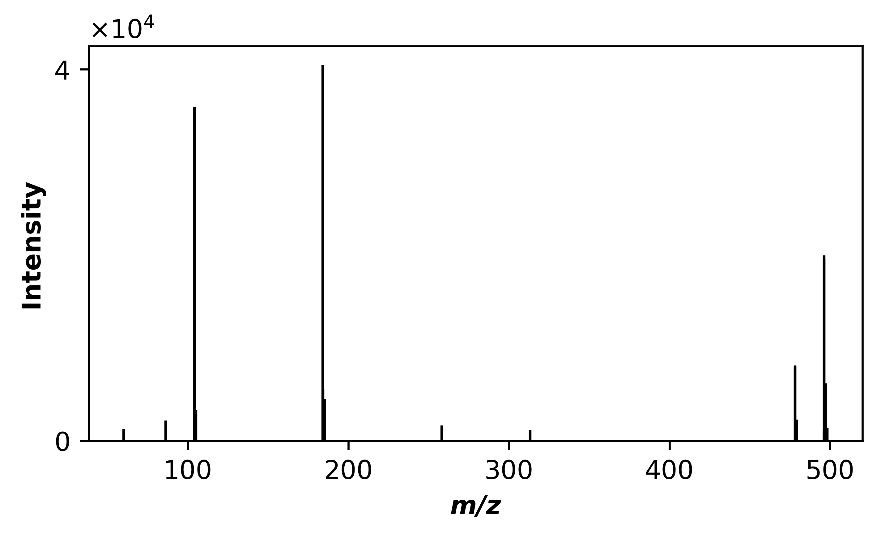
Visualize fragmentation spectra of the highest intensity MS1 feature:

deimos.plot.stem(np.array(res.loc[61, 'mz_ms2']),
                 np.array(res.loc[61, 'intensity_ms2']),
                 width=1)
plt.tight_layout()
plt.show()